Lecture 4: Exact Inference
Introducing the problem of inference and finding exact solutions to it in graphical models.
Introduction
In this previous lectures, we introduce the concept of Graphical Models and its mathematical formulations. Now we know that we can use a graphical model $M$ (Bayesian network or undirected graph model) to specify a probability distribution $P_{M}$ satisfying some conditional independence property. In this lecture, we will study how to utilize a graphical model. Given a GM $M$, we generally have two type of tasks
- Inference: answering queries about the probability distribution $P_M$ defined by $M$, for examples, where $X$ and $Y$ are subsets of variables in GM $M$.
- Learning: estimating a plausible model $M$ from data $D$. We call the process of obtaining a point estimate of $M$ as learning, but for Bayesian, they seek the posterior distribution of , which is actually an inference problem. The learning task is highly related to the inference task. When we want to compute a point estimate of $M$, we need to do inference to impute the missing data if not all the variables are observable. So the learning algorithm usually uses inference as a subroutine.
Inference Problems
Here we will study different kind of queries associated with the probability distribution $P_M$ defined by GM $M$.
Likelihood
Most queries one may ask involve an evidence, so we first introduce the definition of evidence. Evidence $\mathbf{e}$ is an assignment of a set of variables $\mathbf{E}$. Without loss of generality, we assume that $\mathbf{E}={X_{k+1}, \cdots, X_k }$.
The simplest kind of query is the probability of evidence $\mathbf{e}$
this is often referred as computing the likelihood of $\mathbf{e}$.
Conditional Probability
We are often interested in the conditional probability of varaibles $X$ given evidence $\mathbf{e}$
this is the a posteriori belief $X$ given evidence $\mathbf{e}$. Usually we only query about a subset of variables $Y$ of all domain variables $X = {Y, Z}$ and “don’t care” about the remaining, $Z$:
The process of summing out the “don’t care” variables $Z$ is called marginalization, and the resulting is called a marginal prob.
A posteriori belief is very useful. Here we show some applications of a posteriori belief:
- Prediction: computing the probability of an outcome given the starting condition.
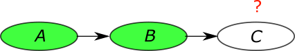
In this type of queries, the query node is the descendent of the evidence. If we know the value of variable $A$ and $B$, the probability of the outcome is a posteriori belief . Using the conditional independence encoded in the graph, we can simplify it to .
- Diagnosis: computing the probability of disease/fault given symptoms.
In this type of queries, the query node is the ancestor of the evidence. In the GM $M$, if we know the value of variable $B$ and $C$, the probability of the cause is a posteriori belief . Again using the conditional independence, we can simplify it to .
- Learning: when learning with partial observation of the variables, we need to compute a posteriori belief in the learning algorithm. In EM algorithm, we will use a posteriori belief to fill in the unobserved variables as part of the algorithm. We will cover more details about learning algorithms later.
The information flow between variables is not restricted by the directionality of the edges in a GM.
We can actually do a probabilistic inference combing evidence from all parts of the networks.
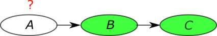
Deep Belief Network (DBN) [Hinton, 2006]
Most Probable Assignment
Another interesting query is to find the most probable joint assignment(MPA) for some variables in interest. Such reasoning is usually performed under some evidence $\mathbf{e}$ and ignoring some “don’t care” variables $Z$,
From the equation, we can find that MPA is the maximum a posteriori configuration of $Y$.
This query is typically useful for prediction given a GM $M$.
- Classification: find the most likely label, given the evidence.
- Explanation find the most likely scenario, given the evidence.
Important Notice: The MPA of a variable depends on its “context” of the problem — the set of variables been jointly queried. For example, the probability distribution of $y_1$ and $y_2$ is shown in the following table. When we compute the MPA of $y_1$, we first compute the marginalization $p(y_1=0) = 0.4, p(y_1=1) = 0.6$, MPA is $\arg \max_{y_1} p(y_1) = 1$. On the other hand the MPA $y_1, y_2$ is $\arg \max_{y_1, y_2} p(y_1, y_2) = (0, 0)$.
| $y_1$ | $y_2$ | $p(y_1, y_2)$ |
|---|---|---|
| 0 | 0 | 0.35 |
| 0 | 1 | 0.05 |
| 1 | 0 | 0.3 |
| 1 | 1 | 0.3 |
Inference Methods
Inference is generally a hard problem. Actually, there is a theorem showing that computing $P(X = \mathbf{x} | \mathbf{e})$ in a GM is NP-hard. However, the NP-hardness does not mean that we cannot solve inference. The theorem implies that we cannot find a general inference procedure that works efficiently for arbitrary GMs. We still have a chance to find provably efficient algorithms for some particular families of GMs.
There are many approaches for inference in GMs. They can be divided into two classes
- Exact inference algorithms. Including the elimination algorithm, message-passing algorithm (sum-product, belief propagation), the junction tree algorithms. These algorithms can give the precise result of query. The major topic of this lecture is on exact inference algorithms.
- Approximate inference techniques. Including stochastic simulation / sampling methods, Markov chain Monte Carlo (MCMC) methods, variational algorithms. These algorithms only gives an approximate answer to the inference query. We will cover these methods in future lectures.
Elimination Algorithm and Examples
Now that we understand the problem of inference, we will examine some simple cases to build intuition for a general method for exact inference.
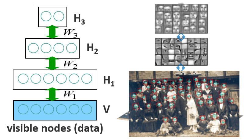
Elimination on Chains
Consider a simple chain on variables $A, B, C, D, E$ as seen below.
Imagine we want the probability of $E=e$ regardless of the values of $A, B, C, D$. Naively, we could sum over the joint probability:
This will require an exponential number of terms. Thankfully, we can use the properties of Bayesian Networks to cut down on this computational cost. Since Bayesian Networks encode conditional independences, we can decompose the joint probability as follows:
This decomposition has allowed us to decouple conditionally independent variables and we can therefore push in and isolate summations, like the following:
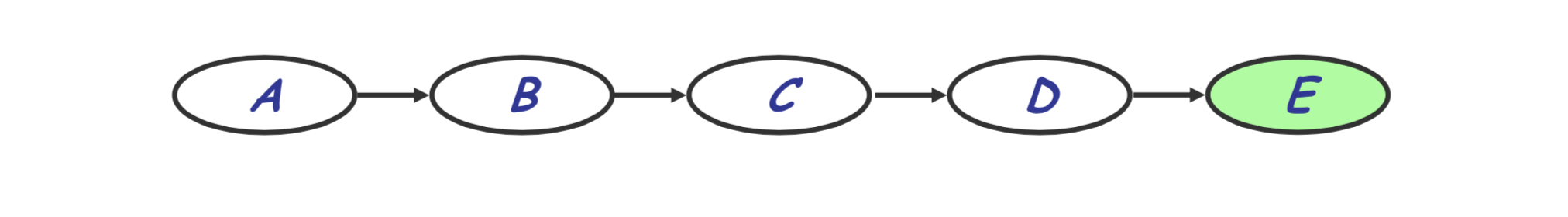
Focusing on the final term, $\sum_a P(a)P(b\vert a)$, we see that this marginalizes over $a$ and leaves us with a function of only $b$. We will generally refer to this as $\phi(b)$ but semantically it is equivalent to $P(b)$. We are left with the following expression for the marginal probability of $e$.
Note that because the variable $a$ is no longer part of this expression we will say $a$ has been eliminated. We are therefore left with a new graphical model for our situation:
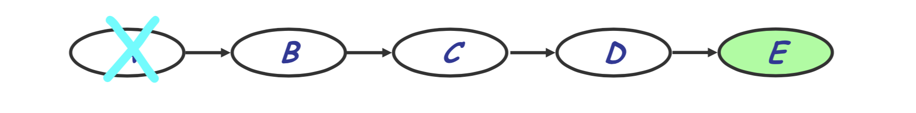
Repeating this, we get the following sequence of steps:
As each elimination step costs $O(Val\vert X_i \vert \times \vert X_{i+1} \vert)$, the overall complexity is $O(nk^2)$, a huge improvement overall from the exponential runtime of the naive summation of the joint probability.
Elimination in Hidden Markov Models
Now we will consider a model frequently used in time-series analysis and Natural Language Processing known as a Hidden Markov Model.
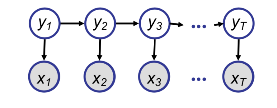
Naively we could find the conditional probability of $y_i$ given the observed sequence, but using our elimination trick, we can get similar computational advantages as seen in the chain example.
With this model, we have two intuitive choices for the order of variables to eliminate. We could start from the first time step (known as the Forward Algorithm) or start from the final time step (known as the Backward Algorithm).
Note that to each notation, we will represent a summation over all random variables $y$ except the $i$th variable as $y_{-i}$.
Forward Algorithm
If we choose to eliminate variables by starting at the beginning of the chain, we would first group factors as follows:
We can continue in this pattern with each intermediate term $\phi(\cdot)$ representing a joint probability.
Backward Algorithm
If we choose to eliminate variables by starting at the end of the chain, we would first group factors as follows:
We can continue in this pattern with each intermediate term $\phi(\cdot)$ representing a conditional probability.
Takeaways from Examples
The main takeaways from our exploration are that elimination provides a systematic way to efficiently do exact inference and that while we can generally create intermediate factors, the semantics of the intermediate factors can vary.
Variable Elimination Algorithm
From these examples, we can consolidate our techniques used in the above examples to a more general algorithm called Variable Elimination.
Note that a frequent operation in the above examples is that of taking a product of factors ($F$) and then summing over the values of a variable. This is the general Sum-Product operation.
Furthermore, we would like a way of incorporating evidence $E=e$ that generalizes our use of factors above. Because we will be maintaining a list of factors and iterating through it, it will be advantages to define new factors that explicitly incorporate our evidence, instead of having fixed variables inside our original factors.
Let $\delta(E_i, e_i)$ denote our evidence potential.
Then as fitting with out existing framework, we can simply define the total evidence potential to be the product our each of the individual evidence potentials.
Now we can treat evidence as just another type of factor.
With these concepts in hand we can outline our new algorithm.
- Given a query of the form $P(X_1 | e)$, we first focus on the joint probability $P(X_1, e)$. . This suggests an implicit “elimination order” over the variables.
- Following the order prescribed above:
- Move all the relevant terms to the innermost sum and all irrelevant terms out of it.
- Perform the Sum-Product operation on the innermost sum, producing a new factor $\phi$.
- Repeat until the entire joint is calculated.
- So calculate the desired query, simply divide the joint by the marginal probability of the evidence.
Graph Elimination
In this section we are going to analyze the complexity of Variable Elimination (VE) algorithm. We first give a basic analysis based on the algorithm procedure and this can give us the insight of the bottleneck of complexity. Then we show that each step of VE can be viewed as a graph transformation step and this can let us analyze the algorithm complexity more clearly in graph perspective. We also formalize the graph perspective view of VA as graph elimination algorithm.
Basic Complexity Analysis
From last section we have known VE can reduce inference complexity greatly. Now let’s have a closer look. Let $n$ be the number of variables in the fully joint probability, $m$ be the number of initial factors including original factors and evidence potentials. We have seen that VE is an n-step iterative elimination algorithm. In each step the algorithm picks a variable $X_i$ and “push in” the summarization w.r.t. $X_i$, which makes the summarization performs over the product of only a subset of factors involving $X_i$. Let $N_i$ be the number of variables ($y_1, y_2, …, y_{N_i}$) inside the subset of factors. We can formally write the step as:
Where $k_i$ is the number of factors involving $X_i$.
Assume each variable has no more than $v$ values, for each configuration of $y_1,…,y_{N_i}$ there is $\textnormal{Val}(X_i) k_i \le v N_i$ multiplication and $\textnormal{Val}(X_i) \le v$ addition. And there are at most $v^{N_i}$ configurations of $y_1,…,y_{N_i}$. Considering the algorithm has $n$ steps, and let $N_{max} = \max_i N_i$. We can write down the complexity is $O(nv^{N_{max}})$. Thus we see that the computational cost of VE algorithm is dominated by the maximum size of intermediate factors generated in an exponential growth rate.
VE to Graph Elimination: Example
We have seen the bottleneck of the VE algorithm is the maximum size of intermediate factors. It is affected by the elimination ordering. Now let’s first see an example that connects iterative elimination steps inside VE with a series of graph structure transformations. This gives us a visualization way of analyzing complexity based on graph elimination. Questions regarding the computation complexity of the VE can be reduced to purely graph-theoretic considerations.
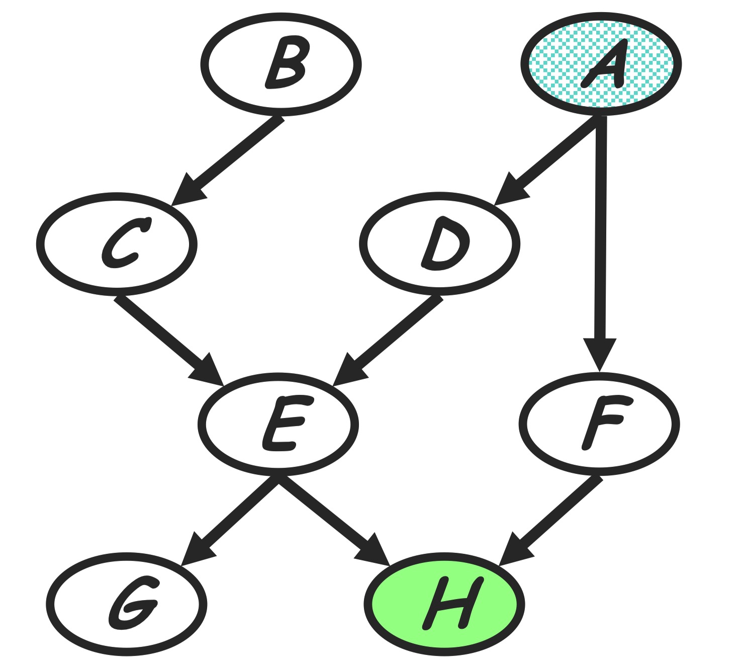
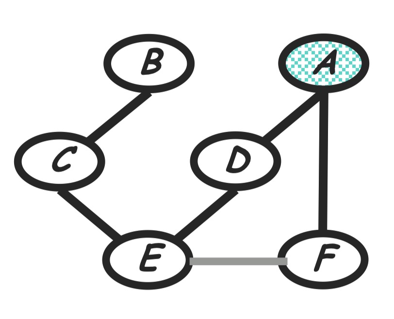
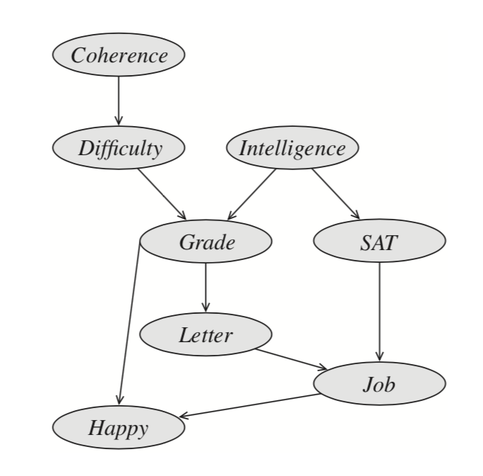
| Given a Bayesian Network factorizing as the graph shown in below, we are going to do VE to inference $P(A | h)$. The initial factors are: |
Before doing VE we choose an elimination ordering as $H,G,F,E,D,C,B$.
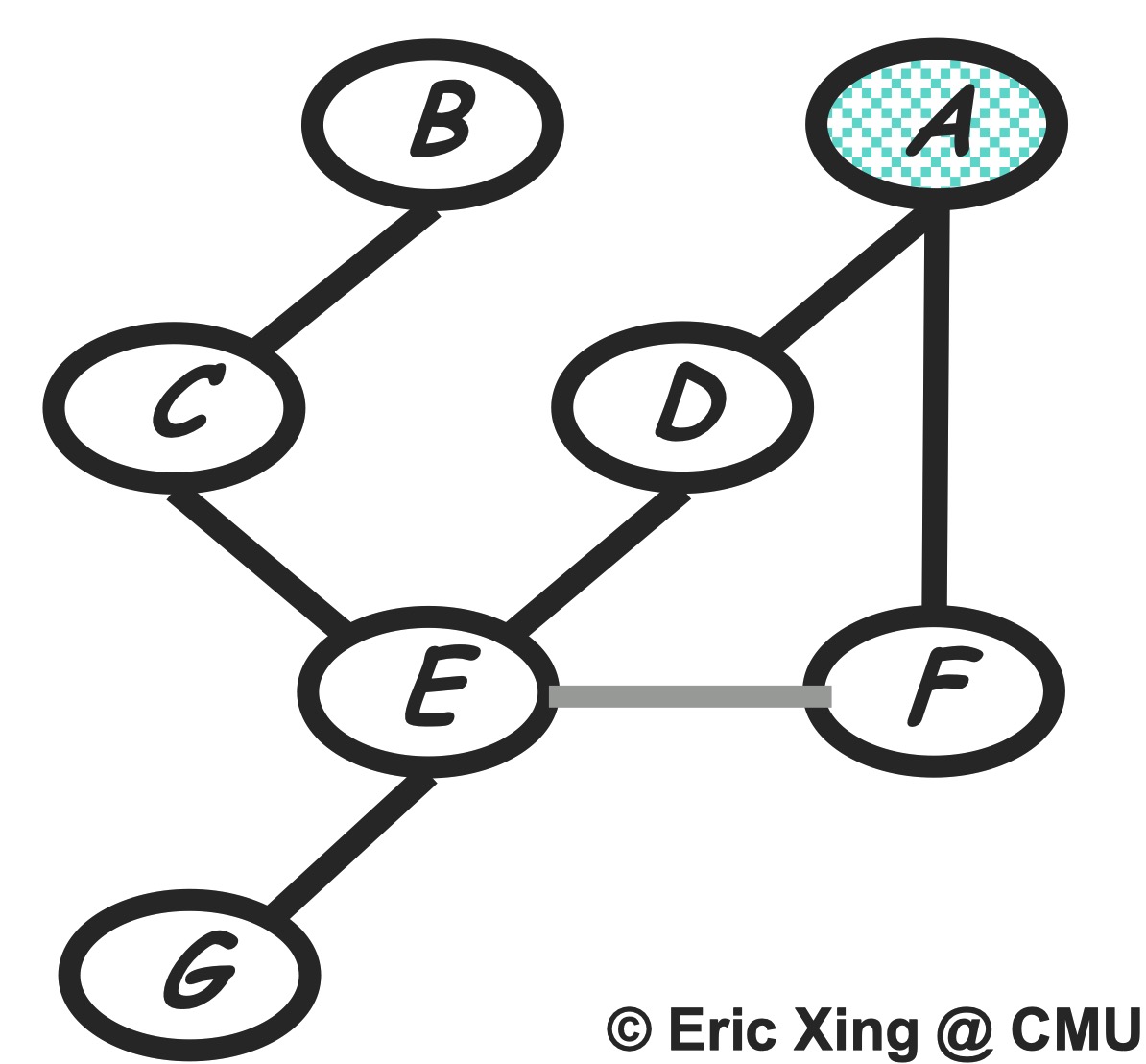
Step 1: to handle conditioning $h$
H variable node is observed node, we can add additional evidence indicator factor to make conditioning on observed evidence as isomorphic as a marginalization step:
The new product of factors becomes:
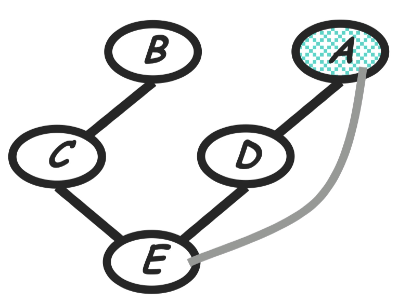
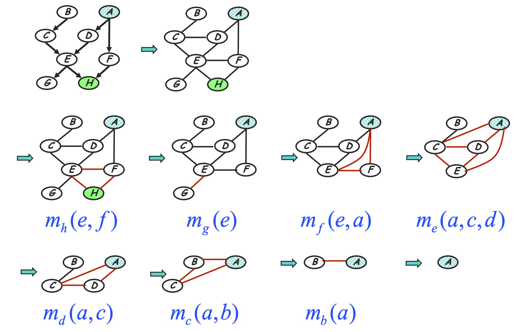
Graph transformation: After conditioning on $h$, we eliminate $h$ in old factors and generate a new factor $m_h(e, f)$. In the perspective of graph evolving, as shown in the below, this corresponding to delete the node $h$ as we eliminate $h$, and also add an edge between node $E$ and $F$ since the generated new factor depending on $E$ and $F$. The reduced factorization is a Gibbs distribution factorizing over the new graph.
Step 2: eliminate G
Compute:
The new product of factors:
Graph transformation: Just remove node $G$ as the below.
Step 3: eliminate F
Compute:
The new product of factors:
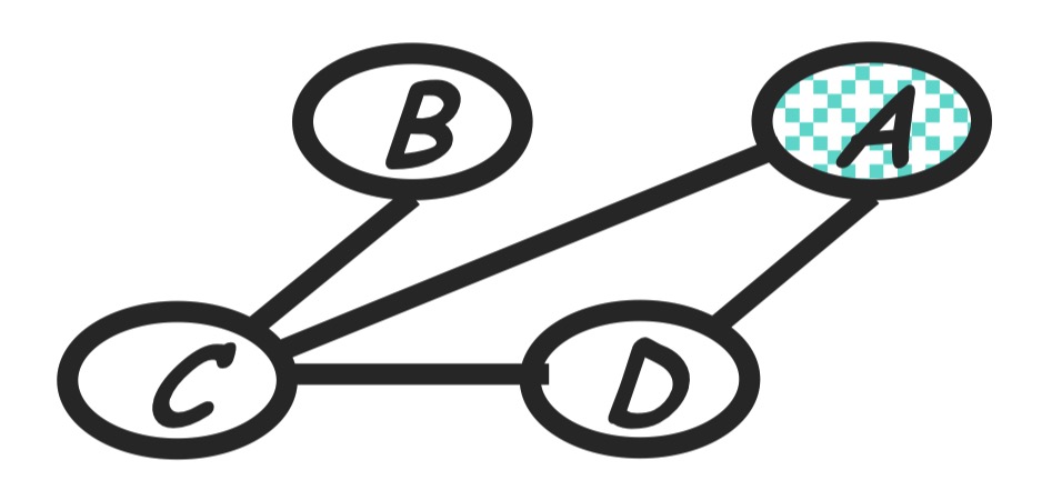
Graph transformation: Remove node $F$ and moralize $A$ and $E$.
Step 4: eliminate E
Compute:
The new product of factors:
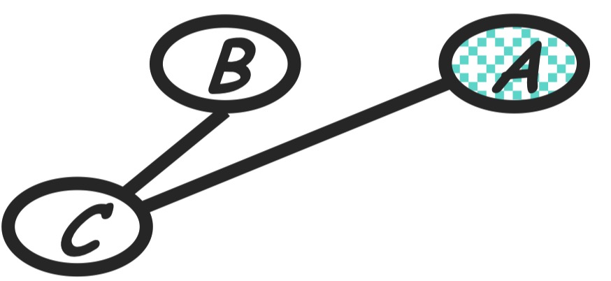
Graph transformation: Generated term <=> fully connected subgraph, according to the Gibbs distribution property. As shown in the follwing, node $E$ is removed and $E$’s neighbors are moralized.
Step 5: eliminate D
Compute:
The new product of factors:
Graph transformation: As in the following.
Step 6: eliminate
Compute:
The new product of factors:
Graph transformation: As in the following, moralize $A$ and $B$.
Step 7: eliminate B
Compute:
The new product of factors:
Graph transformation: Now only a single node $A$ left.
In the last step we just normalize left product.
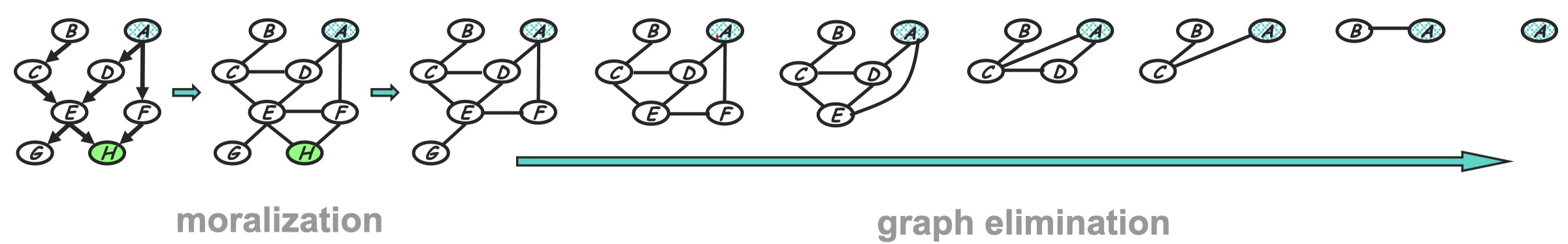
All in all we can see the corresponding graph transformation can be shown as following. At each step we remove a node from the former graph and moralize removed node’s neighbors.
VE to Graph Elimination (GE): Formal Connection
As we have shown in the above example, intuitively the graph elimination procedure has a close connection with variable elimination algorithm. We first summarize the graph elimination algorithm, give out the definition of an important graph structure reconstituted graph, and a theorem about the correspondence of elimination clique in GE and the generated intermediate term in VE.
Graph Elimination Algorithm :
Given: undirected/directed graph $G$, an elimination ordering $I$.
Initialization: If $G$ is directed, first moralize $G$.
Procedure: For each node $X_i$ in $I$, at each step connect all of the remaining neighbors of $X_i$ and remove $X_i$ from the graph.
Reconstituted Graph $G’_I(V, E’)$: also named induced graph
Note: the $I$ is an elimination ordering, for different $I$ reconstituted graph is different.
Definition: the reconstituted graph $G’_I(V, E’)$ is a graph whose edge set $E’$ is a superset of $E$ containing all edges of $E$ and any new edges created during a run of Graph Elimination Algorithm.
Reconstituted graph records the elimination cliques created in graph elimination algorithm. At each step before we remove a node $X_i$ from graph, connecting all neighbors of $X_i$ created a clique, which is the elimination cliques
Correspondence between intermediate terms in VE and elimination cliques in GE:
Following the corresponding steps of VE and GE, it’s easy to see that at each elimination step, the scope of generated intermediate term in VE is just he elimination clique generated in GE. The following figure shows this relationship based on the example we introduced before:
Theorem:
-
The scope of every factor generated during the variable elimination process is a clique in reconstituted graph $G’_I(V, E’)$.
-
Every maximal clique in reconstituted graph $G’_I(V, E’)$ is the scope of some intermediate factor in the computation.
The proof of the theorem can be found in Chapter 9 of Koller’s PGM textbook. This theorem tells us the scope of intermediate factors which is a elimination clique, is a clique in reconstituted graph. What’s more, the scope of the largest intermediate factor is a the largest maximal clique in reconstituted graph.
Complexity Analysis in Graph Perspective
In the beginning of this section we have argued that the bottleneck of VE’s complexity is determined by the scope size of the maximum intermediate factor generated in the procedure of VE. In above subsection we have shown that each intermediate factor in VE is an elimination clique in graph elimination algorithm, and the largest elimination clique is also a largest maximal clique in reconstituted graph.
Then, given an elimination ordering $I$, the problem of get the bottleneck maximum scope size $N_{max}$ of intermediate factors is equivalent of finding the largest clique in reconstituted graph $G’_I(V, E’)$, which is a pure graph theoretic question. And there are efficient mature algorithm for solving this problem.
Elimination Ordering
We can define the width of a reconstituted graph as the size of largest clique minus 1. Let $w_{G,I}$ be the width of $G_I’(V, E’)$. For different ordering $I$, $w_{G,I}$ is different.
Now we define tree-width of $G$ as:
This term provides us a bound on the best performance we can hope for applying VE to do an inference over a probability that factorizes over $G$.
However, finding the best elimination ordering of a graph is a NP-hard problem. As we have shown before the inference task itself is also NP-hard. But these two NP-hard problems are not same. To be more specific, even we have find a best elimination ordering, the complexity of inference can still be exponential if the tree width of the graph $G$ is large.
Although design a general best elimination ordering finding algorithm is NP-hard, there are some heuristic algorithm can generate a near-optimal elimination ordering (look at Koller’s PGM for detail). And on the other hand, for some particular graph $G$ there exists “obvious” optimal ordering that can be easily got. Now we give some examples to show opposite scenarios.
Example 1: Star graph
If we remove centroid first it’s easy to see the width of induced graph is equal to $N-1$ where $N$ is total number of nodes. However if we remove centroid at the end, it’s easy to see the induced graph is the original star graph and the width is just 1. Using this elimination ordering can make variable elimination very efficient.
Example 2: Tree graph
It’s obvious that eliminating nodes from leaves to root won’t introduce any induced dependency so the induced graph is just the original tree. And we know that there is no clique with size large than 3 in tree. So the width is just 1.
Example 3: Ising model
It’s extremely hard to find a optimal elimination ordering. And actually the tree width of ising model is large than the $\sqrt{n}$ so even finding a optimal elimination ordering, the VE algorithm is still exponential in $n$.
Message Passing Algorithms
Overview
Now we have devised a general Eliminate algorithm that is able to work on every graph. However, it has several downsides. One of them, as we have discussed, is exponential worst case complexity. Another one is that it is designed to only answer single-node queries. In this section, we build on the same idea of exploiting local structure of a graph to manipulate factors, and formulate a class of exact inference algorithms based on passing messages over the Clique tree data structure. Doing so will give us important insight on the way inference works in general, and also provide computational benefits in the case when multiple queries have to be computed based on the same evidence. Next, we will show that the message-passing idea can be implemented more efficiently for the special case tree-like graphs. Finally, we conclude with a summary of exact inference.
This section will provide just a cursory overview of the aforementioned techniques, with the intent of presenting intuitions about how they connect to one another, and also clearing up some confusing terminology. For more in-depth explanations and proofs for each of the topics, the scribe would advise looking into the references.
Variable elimination and Clique Trees
Let us start by drawing a connection between variable elimination process as we have seen in Eliminate algorithm, and a special data structure called a Clique tree (also known by the names of Junction or Join tree). Recall that performing one step of variable elimination involved creating a factor $\psi_i$ by multiplying several existing factors, and then one variable is summed out of $\psi_i$ to create a factor $\tau_i$ that is sent to other factors as a “message”. A run of this algorithm defines a Clique tree: it is an undirected graph with nodes corresponding to factors $\psi_i$, or cliques of variables $C_i$ in its scope; an edge between $C_i$ and $C_j$ is added if a message $\tau_i$ is used to in the computation of $C_j$’s message $\tau_j$. Notice that any message $\tau_i$ is passed only once: when a factor $\phi_i$ is used to create the next factor $\psi_j$, it is never used again; hence this graph can be seen to be a tree. Figures below present an example.
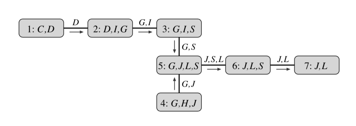
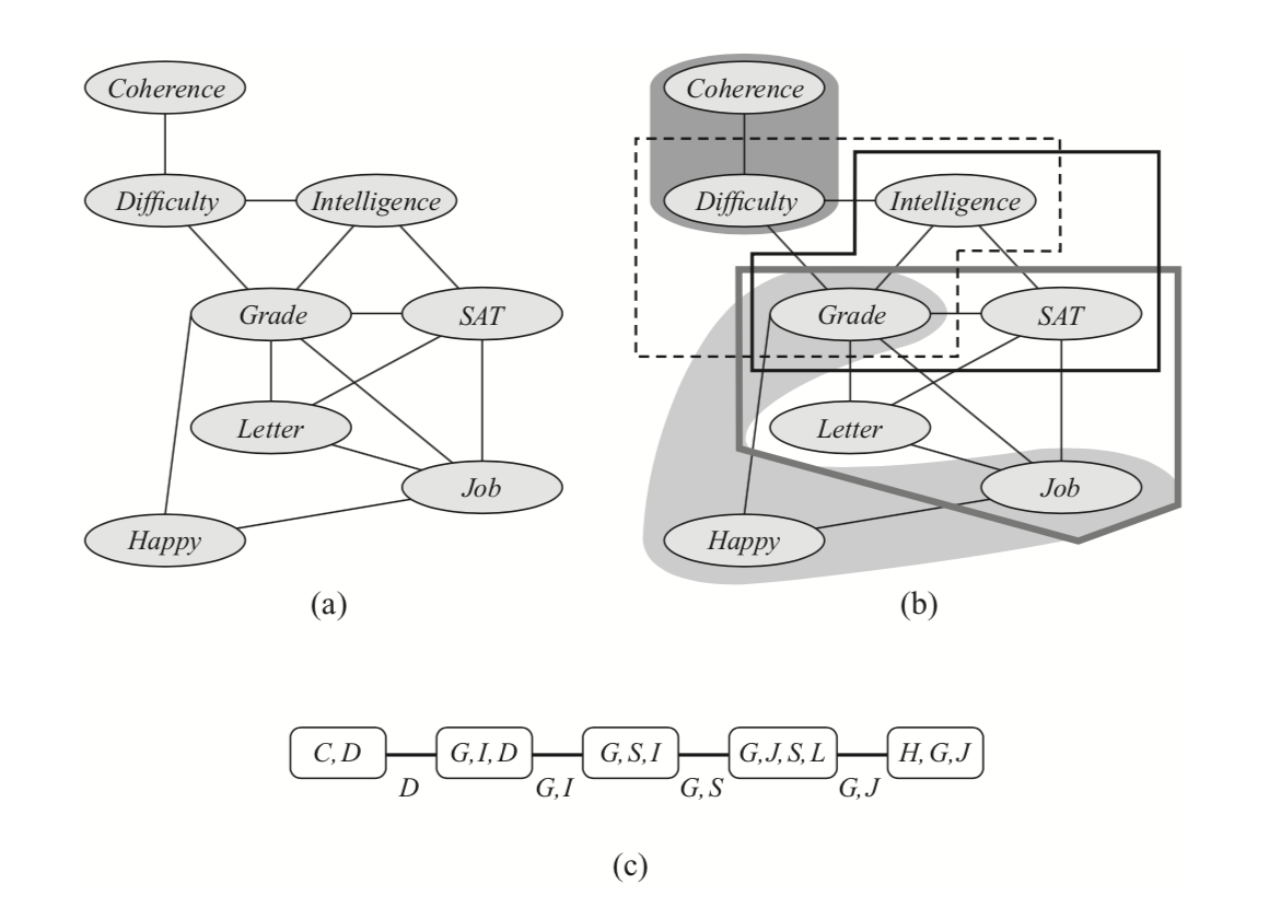
A more algorithmically principled way of constructing a clique tree given the elimination order triangulates $\mathcal{G}$ into its chordal graph, extracts max cliques in it and and finds a minimal spanning tree in the resulting clique graph. Triangulation “triangulates” the graph by iteratively adding an edge between any non-adjacent vertices into any cycle of length at least $4$. Equivalently, given elimination order, we can add edges that would be added if we were to run elimination. Next, maximal cliques $C_i$ are extracted from this graph and arranged in a graph with edges $s_{i,j} = C_i\cap C_j$. Finally, a minimum spanning tree in this graph is a clique tree. The initial graph, triangulated graph, max cliques and the corresponding clique tree are presented in the below example.
Moreover, there is a simple characterization of exactly those trees with $C_i \subseteq X$ as nodes and $S_{i,j} \subseteq C_i\cap C_j$ as edges that are clique trees defined by some variable elimination procedure (using a property called Running Intersections). This lets us identify clique trees with executions of variable elimination. As we will see, interpreting variable elimination in terms of clique trees has several computational advantages. For example, one tree may be used as a basis for executing several different elimination orderings. Furthermore, it makes it possible to cache intermediate messages for answering multiple marginal probability queries more efficiently.
General Sum-Product on a Clique Tree
The Sum-Product algorithm provides a way to use a Clique tree to guide variable elimination. Starting with a clique tree $\Tau$ with cliques $C_i$, we perform the following steps:
- Generate initial potentials by multiplying factors assigned to each clique $C_i$:
- Choose root $C_r$ to be a clique that contains variable of interest.
- Orient the graph upward towards the root. This defines partial ordering of operations on the tree.
- Pass messages bottom-up (collect evidence phase): in the topological order from leaves to root, compute and store
- Distribute messages top-down (distribute evidence phase): for each clique $C_i$
After step $4$, we can get the marginal for the root node, $P(C_r)$, by multiplying the incoming messages with $C_r$’s own clique potential:
(to get the likelihood of the variable of interest, it remains to sum out irrelevant variables). However, the benefit of using the clique tree shows after the top-down phase of step $5$, after which the beliefs $\beta_i$ we obtain are actually equal to marginals $P(C_i)$ for every clique. This way, running $N$ marginal queries is reduced from $Nc$ to just $2c$ (at the cost of storing the tree and messages between bottom-up and top-down passes).
There are several modifications of the algorithm. One replaces sum-product with max-product in the collect evidence phase, and with traceback in the distribute evidence phase, to produce a MAP estimate for $\mathcal{G}$. Another gives a way to do posterior sampling on from the model, by having the collect evidence phase proceed as usual, and on the distribute evidence phase sampling variables given the values higher up the tree.
The resulting Clique (Junction) tree algorithm is a general algorithm for exact inference. However, it inherits the worst-case complexity of the Eliminate algorithm, which is exponential in the size of the largest clique in elimination order. The smallest size of largest clique over all elimination orderings is called the treewidth of a graph; it captures the complexity of VE, as well as CTA. However, finding the ordering, as well as the treewidth itself, is NP-hard in general. This limits the applicability of both of these algorithms.
Next, we will present a more specialized instantiation of a message-passing algorithm that is limited to trees or tree-like structures, but is more efficient. Moreover, it can be applied to non-trees in an iterative fashion, resulting in an approximate inference algorithm known as Loopy Belief propagation.
Sum-Product algorithm on trees
There is a special class of models for which the exact inference can be performed especially efficiently. If $\mathcalP{G}$ is a undirected tree or a directed graph whose moralization is an undirected tree, we can use the Sum-Product message passing in the same way as described before, using the graph itself in place of a clique tree. Likewise, max-product variation for MAP inference and posterior sampling can both be used; moreover, the algorithm can be extended to certain tree-like structures through construction of so called Factor graphs. This algorithm is also known as Belief Propagation, and when applied to chain graps, as Forward-Backward algorithm. This multitude of names reflects the practical significance of this algorithm: although it is limited to certain graphical model structures, it is efficient due to low treewidth of those models and not needing to construct a clique tree in order to obtain all singleton marginals.
One more interesting feature of the tree Sum-Product algorithm is that we can still apply it to graphs that are not trees (i.e. have loops) by repeatedly running message passing until convergence: in that case, it yields an approximate inference method. This algorithm is called Loopy Belief Propagation, and it has been experimentally shown to work well for different classes of models.
Summary of exact inference
Let us recap what we have learnt about exact inference. We have seen Eliminate, Clique tree, and Sum-Product algorithms. Eliminate algorithm is conceptually simple and applicable to any graphical model. However, it only lets us compute single queries and has worst case exponential time complexity in treewidth. Clique tree algorithm is also applicable to general graphs and is able to fix the first of Eliminate’s issues by caching computation using messages, but has the same computational complexity as a function of graph properties. Sum-product algorithm can be thought of as implementing the same idea of passing messages around the graph and can thus be for several-query applications, but reduces the computational complexity of Clique tree algorithm at the cost of being limited to tree-like graphical models.
In general, the above trade-offs between generality and computational complexity are unavoidable: it can be shown that exact inference is NP-hard